25 Tips & Tricks in Excel of Making you a specialist and increasing Efficiency

 

25 Tips & Tricks in Excel of Making you a specialist and increasing Efficiency. Absolutely never use Succeed again without knowing these 25 hints and works:

(1) Importing data from websites in Excel

Importing data from websites in Excel, you can connect to multiple data sources, text files, other Excel files, databases & websites.

• Select 'Data' > Get & Transform > From Web
• Press CTRL+V to paste the URL into the text box, then select OK

(2) Sparklines in Excel

In Excel Sparklines allow you to insert mini charts inside any cell and provide a visual representation of data! Use sparklines to show trends or patterns in data. On the 'Insert tab', click 'Sparklines'

(3) Goal Seek in Excel with example

Get fast answers with Goal Seek. It is also known as What-if-Analysis.

Goal Seek basically uses trial & error to back-solve a problem, by plugging in guesses until it arrives at the correct answer.

(4) Conditional Formatting in Excel

Conditional formatting in Excel helps to visualize data and shows patterns & trends in your data.

Select 'Home' > Conditional Formatting > Highlighting Cell Rules

(5) How to use Wildcards in Excel

Wildcards are special characters that allow you to perform partial matches in your Excel formulas.

Excel has three wildcards: 
• tilde ( ~ )
• asterisk ( * ) 
• question mark ( ? )

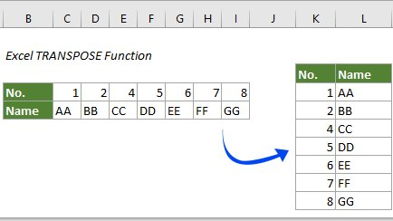
(6) Transpose in Excel

Transpose in Excel will transform items in rows, to instead be shown in columns (or vice versa). Here is an example how to use transpose in Excel.

To transpose a column to a row:

• Select the data in the column

• Select the cell you want the row to start 

• Right-click, choose to paste special, select transpose

(7) Duplicate in Excel

Duplicate in Excel data from the cell above.
• Ctrl + D fills and overwrites a cell with the contents of the cell above it

(8) Remove Duplicates in Excel Sheet

Remove duplicates in a set of data in Excel Sheet. 

• Use the shortcut: Alt + A + M

(9) Filter in Excel

A Filter allows you to filter data. You can filter a column to show a specific product or date.

You can also sort in ascending or descending order.

(10) How to use Slicer in Excel with example

Slicers provide buttons that you can click to filter tables, or PivotTables

Select 'Home', go to Insert > Slicer

(11) How to use Pivot Tables

A powerful tool to calculate, summarize & analyze data, which allows you to compare or find patterns & trends in data.

To access this function, go to "Insert" in the Menu bar, and then select "Pivot Table"

(12) Auto-fill

With large data sets, instead of typing a formula multiple times, use auto-fill. 

There are 3 ways to do this:
• Double click mouse on the lower right corner of the 1st cell, or
• Highlight a Section and type Ctrl + D, or
• Drag the cell down the rows

(13) DatedIf Formula in Excel

Calculates the number of (1) days, (2) months, or (3) years between two different dates

=DATEDIF(X,Y,"D")
X = Start date cell
Y = End date cell 
"D"= Time interval 

• D = Days

• M = Months

• Y = Years

(14) How to use TRIM Formula in Excel

TRIM helps to remove the extra spaces in data.

TRIM can be useful in removing irregular spacing from imported data. 

=TRIM( )

(15) Index Match Formula in Excel

The main difference between VLOOKUP and INDEX MATCH is the column reference

VLOOKUP uses a static column reference but INDEX MATCH uses a dynamic column reference

Index Match is much more flexible as you can search by row, or by column, or by both

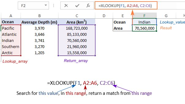
(16) XLOOKUP Formula in Excel

XLookup is an upgrade compared to VLOOKUP or Index & Match.

Use the XLOOKUP function to find things in a table or range by row.

Formula: =XLOOKUP (lookup value, lookup array, return array)

(17) IF function/condition in Excel

The IF function makes logical comparisons & tells you when certain conditions are met.

For example, a logical comparison would be to return the word "Pass" if a score is >70, and if not, it will say "Fail"

An example of this formula would be =IF(C5>70,"Pass","Fail")

(18) Using SUMIF in Excel

Sum the values in a range, if they meet a certain criterion

(19) Using SUMIFS in Excel

Sum the values in a range that meet multiple criteria

Use it if you want the sum of two criteria: Apples & Pete 

Formula =SUMIFS (sum_range, criteria_range1, criteria1, ...)

(20) COUNTIF

Counts the number of cells that satisfy a query. (Count the number of times a word has been mentioned)

(21) COUNTIFS

Counts the number of times a Criteria is met

 
For example, it counts the number of times that both (1) apples and (2) price > $10, are mentioned

(22) UPPER, LOWER, PROPER

• =UPPER, Converts text to all uppercase,
• =LOWER, Converts text string to lowercase,
• =PROPER, Converts text to proper case

(23) CONVERT

This converts one measurement to another. There are multiple conversions that you can do.

An example is metered to feet or Celsius to Fahrenheit.

(24) Stock Market data

You can get stock data in Excel

Enter a list of stock ticker symbols. then select the cells and go to the Data tab, then click the Stocks button within the Data Types group

Excel will attempt to match each cell value to company stock, and fill in the data

(25) Geography / Maps in Excel

Instead of researching geographical data or maps, use Excel

With the Geography data type, you can retrieve data like population, time zone, area leaders, gasoline prices, language, and more

Type the data you need, then go to Data Tab -> Geography

https://talhatahfoor.com/blogs-1/f/%F0%9F%93%8A25-strong-ways-of-making-you-a-specialist